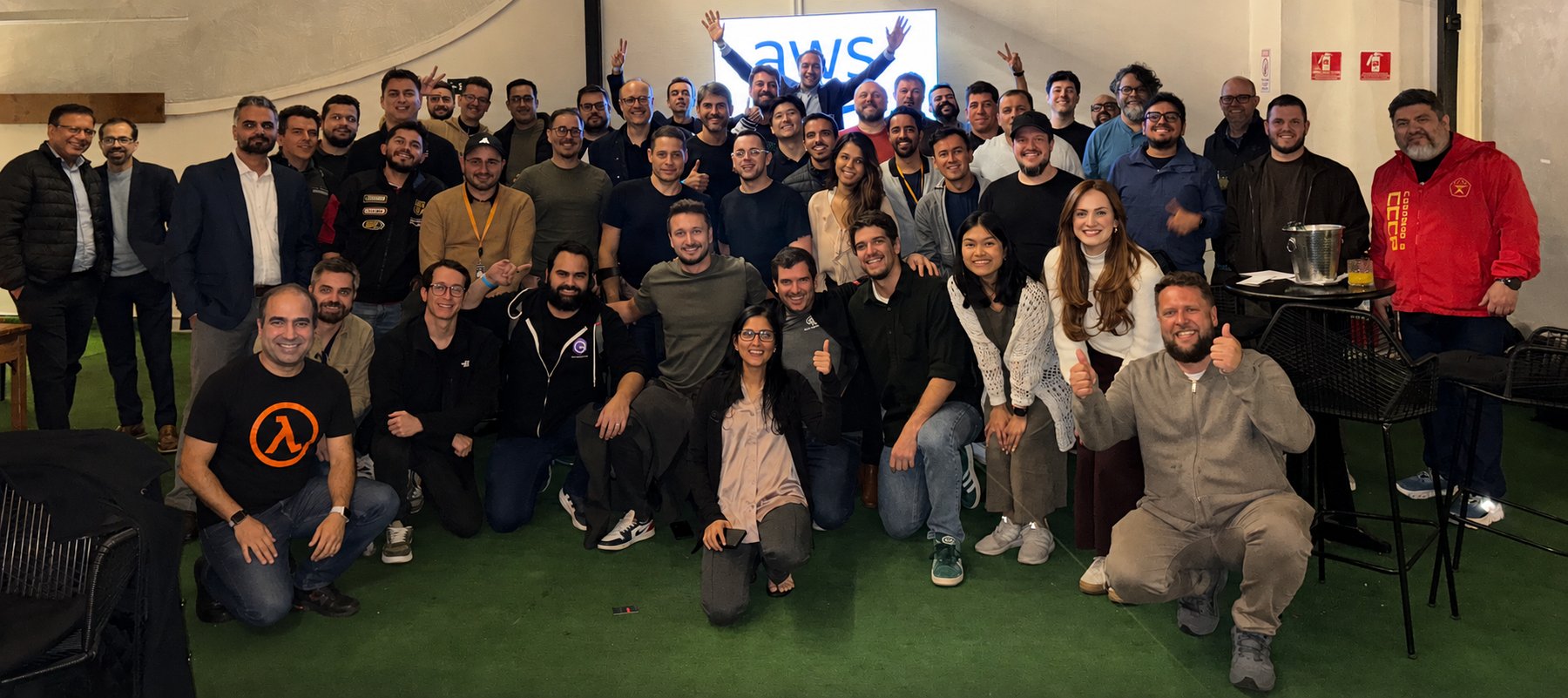
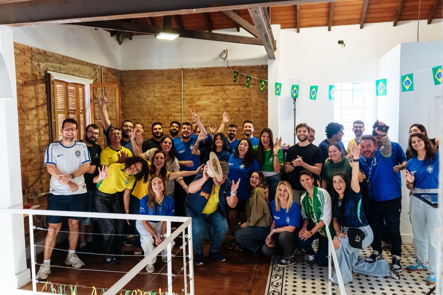
Last week I had the privilege of spending three days in São Paulo with technical builders from across Latin America, brought together for a regional tech event full of deep-dive sessions, hands-on workshops, and conversations with customers and partners. What struck me most wasn’t any single session, it was the energy of a technical community that so rarely gets to be in the same room. People traded architecture ideas over coffee, sketched out solutions on whiteboards, and left with a longer list of things to try than they arrived with. It’s a good reminder that, for all the tooling we build, the community around it is what makes the technology stick.
That community spirit connects nicely to the week’s biggest infrastructure news, which is all about bringing AWS closer to where builders actually are.
Now, let’s get into this week’s AWS news…
Headlines
AWS Local Zone in Athens, Greece: AWS has opened a new Local Zone in Athens, Greece, the second Local Zone in EMEA with support for Amazon S3 and Amazon EBS Local Snapshots, so you can store and process data within Greece to help meet local data residency requirements. The Athens Local Zone supports Amazon EC2 (C7i, M7i, and R7i instances), Amazon S3 with the One Zone-Infrequent Access storage class, Amazon EBS, and Amazon ECS.

AWS Local Zones place AWS infrastructure much closer to large population and industry hubs, enabling applications that require single-digit millisecond latency, such as real-time gaming, media production, and financial services, to run where end users actually are. For builders in Greece, you can now run latency-sensitive workloads locally while connecting seamlessly to the nearest AWS Region for services that don’t require low latency, giving you the flexibility to architect hybrid, latency-optimized applications without managing your own data center infrastructure. To learn more, visit AWS Global Infrastructure and Sustainability Blog post.
Last week’s launches
Here are some launches and updates from this past week that caught my attention:
- Claude Opus 5 on AWS: You can use Anthropic’s Claude Opus 5, the most advanced Opus model yet, matching Claude Fable 5’s top-tier intelligence in many domains at Opus-tier pricing. Amazon Bedrock offers Claude Opus 5 with zero data retention (ZDR) enabled by default, giving you Opus’ top-tier intelligence while meeting your data governance requirements unlike Claude Fable 5. You have two ways to access Claude Opus 5: Amazon Bedrock and Claude Platform on AWS. To learn more, visit the deep dive blog post.
- AWS Lambda durable execution SDK for .NET is now generally available: You can now build resilient, long-running workflows in C# using Lambda durable functions, without implementing custom progress tracking or integrating an external orchestration service. The SDK is a natural fit for multi-step applications like payment processing pipelines, AI agent orchestration, and human-in-the-loop approvals, it checkpoints progress automatically and can pause execution for up to a year. If you’re a .NET developer building serverless workflows, this removes a lot of the plumbing you used to write by hand.
- Amazon Bedrock AgentCore now delivers unified observability with traces and logs in a single log group: Amazon Bedrock AgentCore now delivers agent traces and prompts to the same Amazon CloudWatch log group as your agent’s logs. Previously, telemetry was split across destinations, trace spans went to a shared log group while prompts, inputs, and outputs went to a separate one, so debugging a single agent invocation meant searching in multiple places. You can now debug an invocation in one place, and apply fine-grained access control and customer-managed key (CMK) encryption at the individual agent level.
- Amazon Connect delivers more natural agentic voice experiences: Amazon Connect now supports more natural, human-sounding agentic voice experiences across 50+ languages, including Portuguese, Spanish, French, Italian, Japanese, Korean, and Thai, with over 100 new voice options and conversational improvements that make AI interactions sound more fluid. Connect’s agentic self-service lets AI agents understand, reason, and take action across voice and digital channels, adapting to a customer’s tone and sentiment. You can now build contact center experiences that feel natural to callers in far more of the languages your customers actually speak.
- Amazon SageMaker Unified Studio now supports Amazon OpenSearch: You can now query and analyze your search and log analytics data from Amazon OpenSearch directly alongside other data assets in Amazon SageMaker Unified Studio. With this connection, you can combine operational search data in OpenSearch with data from sources like Amazon Redshift, Amazon S3, and relational databases, all within a single, governed environment. It’s especially useful when you need to correlate analytical and operational workloads, such as joining application logs with transactional data to uncover insights.
- Amazon CloudWatch announces coding agent insights: Amazon CloudWatch now gives engineering leaders visibility into how AI coding tools are driving value across their organization. Coding agent insights integrates with the Claude apps gateway for AWS to collect telemetry from Claude Code without additional instrumentation, and also supports agents like Codex and GitHub Copilot. As teams scale AI coding adoption, you can now measure the return on that investment with metrics built on OpenTelemetry, no custom instrumentation required.
For a full list of AWS announcements, be sure to keep an eye on the What’s New with AWS page.
Other AWS news
Here are some additional posts and resources that you might find interesting:
- Evaluating AI Agents: A production blueprint with Strands and AgentCore: A practical guide to evaluating AI agents before and after they reach production, using Strands Agents and Amazon Bedrock AgentCore. If you’re moving agents from prototype to production, this post is a great companion to the AgentCore observability update above, it walks through how to measure agent quality systematically rather than by gut feel.
- Building multi-region resiliency for AWS CloudFormation custom resource deployment: Learn how to architect CloudFormation custom resources for multi-region resiliency, so your infrastructure-as-code deployments stay reliable even when a single Region has issues.
- Introducing Amazon Simple Email Service (SES) pricing plans: Amazon SES now offers pricing plans that give you more predictable costs as your email volume grows. If you send at scale, this could simplify your billing significantly.
Upcoming AWS events
Check your calendar and sign up for upcoming AWS events:
- AWS Summits: AWS Summits are free events that bring the cloud and AI community together to connect, learn, and explore the latest technologies. Browse the full calendar to find a Summit near you in the second half of 2026.
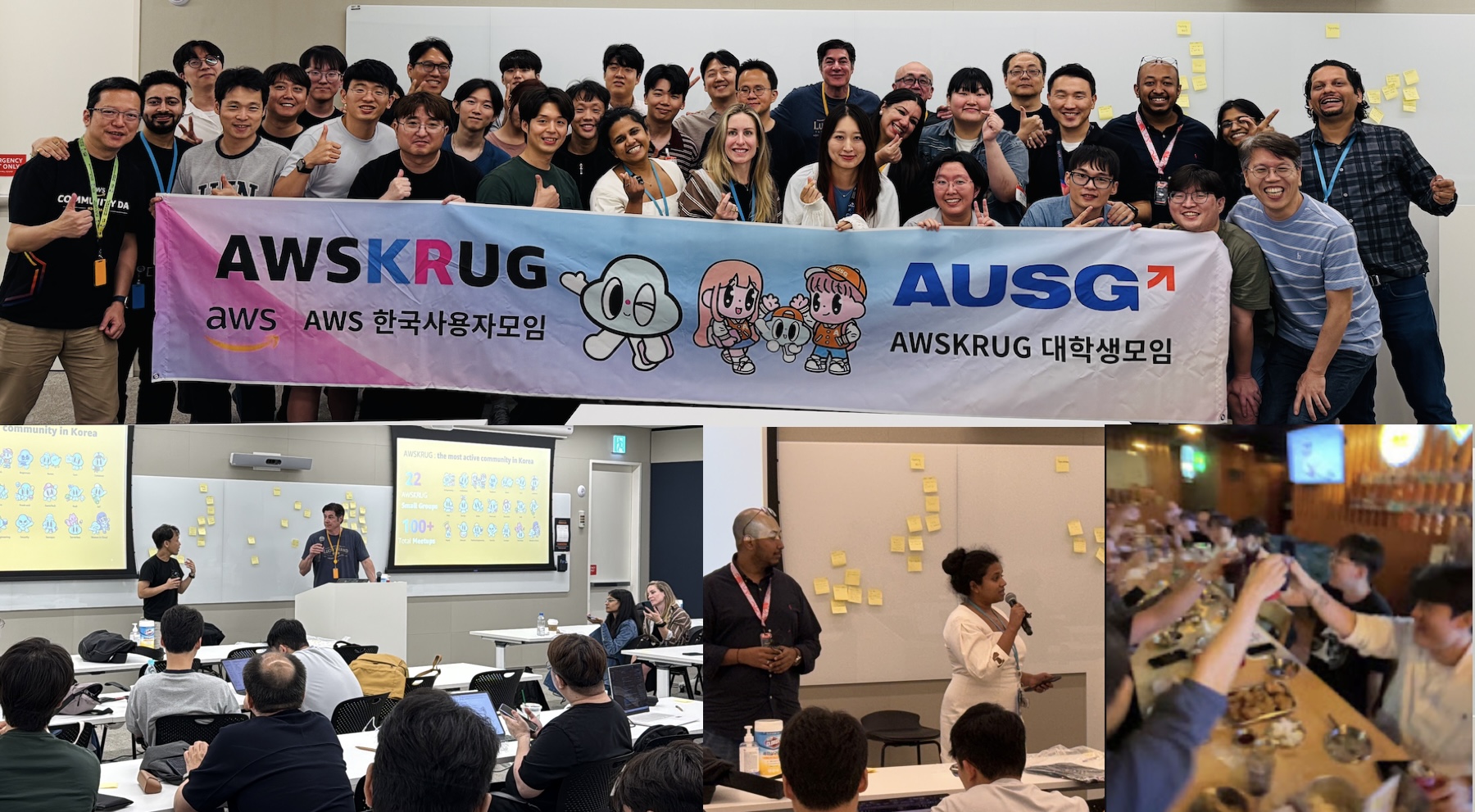
- AWS Community Days: Community-led conferences where content is planned, sourced, and delivered by community leaders. If you’re in Latin America, don’t miss AWS Community Day Belo Horizonte on August 22, registration is open at awscommunityday.com.br.
Join the AWS Builder Center to connect with builders, share solutions, and access content that supports your development. Browse here for upcoming AWS-led in-person and virtual events and developer-focused events.
That’s all for this week. Check back next Monday for another Weekly Roundup!
This post is part of our Weekly Roundup series. Check back each week for a quick roundup of interesting news and announcements from AWS!
from AWS News Blog https://ift.tt/67MGjnO
via IFTTT
 It has been a busy stretch on the AWS Summit circuit. At the